Curve Sketching
Interactive Graph Simulator Available
Explore vectors, limits, or function shifts dynamically side-by-side.
Interactive Graph Simulator Available
Explore vectors, limits, or function shifts dynamically side-by-side.
Interactive Graph Simulator Available
Explore vectors, limits, or function shifts dynamically side-by-side.
Interactive Graph Simulator Available
Explore vectors, limits, or function shifts dynamically side-by-side.
By the end of this session, you will be able to:
- Identify algebraic domain restrictions, axis intercepts, and coordinate symmetry (f(−x)=±f(x)), constructing the foundational pre-calculus framework for analytical curve sketching.
- Calculate vertical, horizontal, and slant (oblique) asymptotes using limit evaluations (limx→c±f(x)=±∞, limx→±∞f(x)=L) and polynomial long division as formalized in Slant Asymptotes and Polynomial Division.
- Apply the First Derivative Test to locate stationary critical points, partition the domain, and establish intervals of monotonic increase and decrease.
- Evaluate the second derivative to determine intervals of upward and downward concavity, locate points of inflection, and classify local extrema via the Second Derivative Test.
- Construct an Information Consolidation Table synthesizing algebraic coordinates with differential rate commands, drafting complete, accurate geometric models using the 3-layer order of operations codified in Summary of Curve Sketching.
📅 Micro-Lecture
1. The Calculus of Shape: Pre-Calculus Blueprint vs. Dynamic Curvature
- Mathematical Foundation: Prior to calculus, graphing functions relied heavily on point-plotting—a brute-force method prone to missing critical turning points, local extrema, or subtle asymptotic behavior. Curve sketching transforms graphing into a rigorous analytical science by decoupling the function into two complementary layers:
- The Pre-Calculus Blueprint: Domain, axis intercepts, symmetry, and boundary asymptotes establish the outer container and coordinate anchors.
- The Differential Anatomy: The first derivative f′(x) establishes slope and direction (↗,↘), while the second derivative f′′(x) establishes curvature and bending (∪,∩).
- Engineering Context: In civil and structural engineering, digital drafting tools and finite-element modeling software do not merely connect discrete points; they evaluate continuous curvature functions. Structural beam deflections, aerodynamic airfoils, and highway cloverleaf ramps require rigorous slope and concavity continuity to prevent catastrophic stress concentrations or vehicle rollover.
2. Asymptotes as Global Boundary Constraints
- Mathematical Foundation: Asymptotes are lines that guide the path of a curve toward extreme limits:
- Vertical Asymptotes (x=c): Occur where output values explode to ±∞ due to zero denominators in rational or logarithmic expressions. A continuous function can never cross its vertical asymptotes.
- Horizontal Asymptotes (y=L): Dictate the end behavior of the function as x→±∞. A curve can cross a horizontal asymptote at finite coordinates; horizontal asymptotes only govern the extreme tails of the domain.
- Slant (Oblique) Asymptotes (y=mx+b): Occur in rational functions when the degree of the numerator is exactly one higher than the denominator (n=m+1). Found via polynomial long division, they describe the linear trajectory the curve approaches at infinity.
- Engineering Context: In electronics, horizontal asymptotes represent power supply voltage saturation rails in operational amplifiers; in chemical kinetics, they represent adiabatic ceiling temperatures in batch reactors.
3. The Anatomy of Concavity and Points of Inflection
- Mathematical Foundation: Concavity measures how the slope itself is changing:
- If f′′(x)>0, slopes are increasing; the curve bends upward like a cup (∪), and all tangent lines lie below the curve.
- If f′′(x)<0, slopes are decreasing; the curve bends downward like a cap (∩), and all tangent lines lie above the curve.
- An inflection point occurs where a continuous curve strictly transitions between concave up and concave down. At this precise point, the tangent line slices directly through the curve.
- Engineering Context: In amusement park design, roller coaster track inflection points mark locations where vertical centripetal acceleration vanishes (an=0), allowing passengers to experience pure, comfortable 1.0 G transitions between high-G valley compressions and zero-G airtime hills.
Skill Block 1
Algebraic Foundations & Asymptotic Boundaries (The Pre-Calculus Blueprint)
General Overview
Skill Block 1 focuses on extracting the geometric skeleton of a function before calculating any derivatives. By systematically auditing domain restrictions, determining axis crossings, evaluating coordinate symmetry, and extracting all vertical, horizontal, and slant asymptotes, students construct the immutable boundary container within which all calculus behavior must operate.
Conceptual Framework
- Domain Restrictions:
- Rational functions: Denominators cannot equal zero (Q(x)=0).
- Even roots: Radicands must be non-negative (g(x)≥0).
- Logarithms: Arguments must be strictly positive (h(x)>0).
- Intercepts:
- y-intercept: Evaluate f(0), producing the unique point (0,f(0)).
- x-intercepts: Solve f(x)=0 for all real roots.
- Symmetry Testing:
- Even Symmetry (y-Axis Mirror): If f(−x)=f(x), the graph is symmetric across the y-axis.
- Odd Symmetry (Origin 180∘ Rotation): If f(−x)=−f(x), the graph is symmetric about the origin.
- Asymptotic Classification:
- Vertical Asymptote (x=c): If limx→c+f(x)=±∞ or limx→c−f(x)=±∞.
- Horizontal Asymptote (y=L): If limx→∞f(x)=L or limx→−∞f(x)=L.
- Slant Asymptote (y=mx+b): For rational functions with deg(numerator)=deg(denominator)+1, use polynomial division to express f(x)=(mx+b)+Q(x)R(x).
Key Equations & Structural Rules
- Symmetry Criterion:
f(−x)=f(x)⟹Even (y-axis),f(−x)=−f(x)⟹Odd (Origin)
- Horizontal Asymptote Rational Degree Rules:
x→±∞limbmxm+…anxn+…=⎩⎨⎧0bman±∞n<mn=mn>m(see Horizontal Asymptotes)
- Slant Asymptote Long Division Formula:
f(x)=(mx+b)+Q(x)R(x)⟹yasymptote=mx+b(see Slant Asymptotes and Polynomial Division)
Worked Example A: Pre-Calculus Blueprint of a Quartic Polynomial
Analyze the algebraic domain, intercepts, symmetry, and end behavior of the polynomial function:
💡 Reveal Worked Solution
- Name the Governing Formulas: The Polynomial Domain Theorem, Axis Intercept Formulas, and Leading Term End-Behavior Test: (These principles are formalized in Summary of Curve Sketching.)
- Determine Algebraic Domain:
Polynomials contain no division by zero, even roots, or logarithms.
Domain: (−∞,∞)
- Calculate Intercepts:
- y-intercept: Set x=0:
f(0)=41(0)4−(0)3=0⟹(0,0)
- x-intercepts: Set f(x)=0 and factor out the greatest common factor x3:
41x4−x3=0⟹x3(41x−1)=0This yields:x3=0⟹x=041x−1=0⟹41x=1⟹x=4The graph crosses or touches the horizontal axis at (0,0) and (4,0).
- y-intercept: Set x=0:
- Test Coordinate Symmetry:
Substitute −x into f(x):
f(−x)=41(−x)4−(−x)3=41x4+x3Comparing to f(x):f(−x)=f(x)andf(−x)=−f(x)The function possesses neither even nor odd symmetry.
- Analyze Asymptotes & End Behavior:
- Asymptotes: None. Polynomial functions have no vertical, horizontal, or slant asymptotes.
- End Behavior: Governed by the highest-degree term 41x4:
x→∞lim(41x4−x3)=∞andx→−∞lim(41x4−x3)=∞Both the far-left and far-right tails rise without bound toward positive infinity (↖,↗).
Practice Problem 1: Concept & Reading Check
Open this Skill Block on the Memex to locate the information needed to answer the following:
- (a) Explain why a function can never cross its vertical asymptotes, but can cross a horizontal or slant asymptote multiple times in the interior of its domain.
- (b) In Worked Example A, explain algebraically why the origin (0,0) is both an x-intercept and a y-intercept.
- (c) In the linked application Highway Interchange Overpass Alignment (Civil Engineering), why is the vertical asymptote at station x=−10 physically irrelevant to the operational roadway?
Review the definitions in Vertical Asymptotes, the algebraic intercept steps in Worked Example A, and question 1 of Highway Interchange Overpass Alignment (Civil Engineering).
Answer: * (a) Vertical asymptotes represent values where the function is strictly undefined (division by zero); horizontal/slant asymptotes only constrain the limit as x→±∞.
- (b) Evaluating f(0)=0 satisfies both the y-intercept condition (x=0) and the x-intercept condition (f(x)=0).
- (c) The physical highway ramp starts at station x=0 (x≥0), so x=−10 lies 1,000 m behind the start of the interchange.
Step-by-Step Execution
- (a) A vertical asymptote occurs at x=c where the denominator vanishes while the numerator is non-zero, making the function value undefined. By definition, no coordinate (c,f(c)) can exist on the curve, so the graph cannot cross a vertical asymptote. In contrast, a horizontal or slant asymptote represents the limiting behavior of the function as x→±∞. The distance ∣f(x)−(mx+b)∣ approaches zero as x grows large, but for finite values of x, f(x) may equal mx+b wherever the remainder term R(x)=0.
- (b) For any function where f(0)=0, substituting x=0 yields an output of 0, establishing (0,0) as the y-intercept. Simultaneously, setting f(x)=0 is satisfied by x=0, making (0,0) a root (x-intercept). The origin is the unique coordinate point in the Cartesian plane that lies simultaneously on both coordinate axes.
- (c) In highway civil engineering, stationing distances are defined along the active physical construction corridor starting at entrance station x=0 (x≥0). Because the singularity x=−10 corresponds to a station 1,000 meters behind the project terminus in the negative direction, the rational function profile is smooth, continuous, and well-behaved across the entire physical project domain [0,∞).
Practice Problem 2
For the rational function:
Set the denominator to zero for the domain. Use synthetic or polynomial long division to divide (x2−x−2) by (x−1) to isolate the linear quotient y=mx+b. (See Slant Asymptotes and Polynomial Division.)
Answer:
Step-by-Step Execution
- Name the Governing Formulas: The Rational Domain Restriction Rule, Intercept Conditions, and Slant Asymptote Long Division Formula: (Defined in Slant Asymptotes and Polynomial Division.)
- Determine Domain:
Set denominator to zero:
x−1=0⟹x=1Domain: (−∞,1)∪(1,∞)
- Calculate Intercepts:
- y-intercept: Set x=0:
f(0)=0−1(0)2−(0)−2=−1−2=2⟹(0,2)
- x-intercepts: Set the numerator to zero and factor:
x2−x−2=0⟹(x−2)(x+1)=0⟹x=2orx=−1Both roots belong to the domain (x=1), yielding intercepts (2,0) and (−1,0).
- y-intercept: Set x=0:
- Evaluate Vertical Asymptote:
At x=1, the numerator is (1)2−(1)−2=−2=0.
x→1+limx−1x2−x−2=0+−2=−∞andx→1−limx−1x2−x−2=0−−2=+∞Thus, the line x=1 is a vertical asymptote.
- Extract Slant Asymptote via Polynomial Long Division:
Divide (x2−x−2) by (x−1):
x−1x2−x−2=x−1x(x−1)−2=x−x−12As x→±∞, the remainder term −x−12→0. Therefore, the slant asymptote is the linear equation:y=x
📅 Regroup 1
- Key Reflection: Why do we factor numerators and denominators before declaring asymptotes? Always check for common linear factors (x−a) that produce removable discontinuities (holes) rather than vertical asymptotes!
- Symmetry Shortcut: If a rational function has an even numerator and an odd denominator, the function is odd (f(−x)=−f(x)); if both numerator and denominator are even, the function is even.
Skill Block 2
Differential Analysis: Monotonicity, Extrema & Curvature (The Calculus Core)
General Overview
Skill Block 2 equips students to analyze the dynamic interior behavior of the curve. By computing the first and second derivatives, constructing 1D sign charts, and classifying critical numbers and inflection points, students determine exactly where the curve climbs, falls, peaks, troughs, and bends.
Conceptual Framework
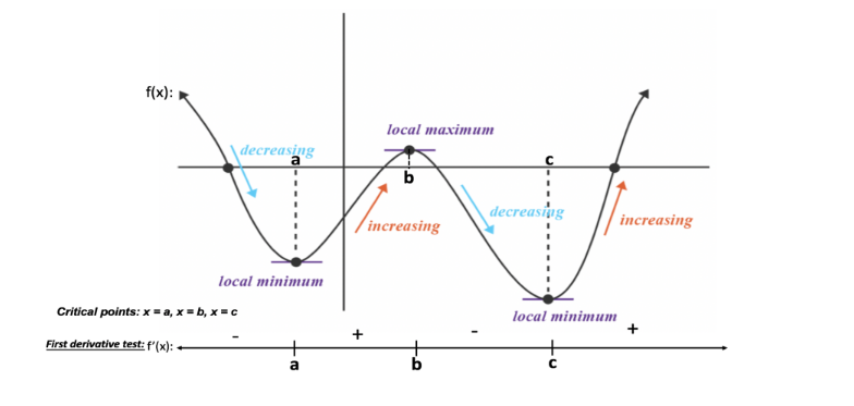
- The First Derivative Test for Local Extrema:
- Locate all critical numbers in the domain where f′(c)=0 or f′(c) is undefined.
- Partition the domain into test intervals.
- Sign of f′(x):
- f′(x)>0⟹ function is strictly increasing (↗).
- f′(x)<0⟹ function is strictly decreasing (↘).
- Extrema transitions:
- +→−⟹ Local Maximum peak.
- −→+⟹ Local Minimum valley.
- The Second Derivative: Concavity & Inflection Points:
- f′′(x)>0⟹ Concave Upward (∪, holds water, slopes increasing, tangent lines lie below).
- f′′(x)<0⟹ Concave Downward (∩, sheds water, slopes decreasing, tangent lines lie above).
- Inflection Point: Continuous coordinate (c,f(c)) where f′′(x) strictly changes sign.
- The Second Derivative Test for Local Extrema:
- If f′(c)=0 and f′′(c)>0⟹ Local Minimum.
- If f′(c)=0 and f′′(c)<0⟹ Local Maximum.
- If f′′(c)=0⟹ Inconclusive (revert to First Derivative Test).
Key Equations & Structural Rules
- First Derivative Test Transition Rules:
f′(x):(+)→(−)f′(x):(−)→(+)⟹Local Maximum at x=c⟹Local Minimum at x=c(see First Derivative Test)
- Concavity & Inflection Criteria:
f′′(x)>0⟹Concave Up (∪),f′′(x)<0⟹Concave Down (∩)Inflection Point at (c,f(c))⟺f′′(x) flips sign across x=c and c∈dom(f)(see Concavity and the Second Derivative Test)
Worked Example A: Differential Analysis of an Odd Cubic Polynomial
Perform a complete differential analysis of the function:
💡 Reveal Worked Solution
- Name the Governing Formulas: The Power Rule for Differentiation, the First Derivative Test for Local Extrema, and the Second Derivative Inflection Criterion: (These principles are formalized in First Derivative Test and Concavity and the Second Derivative Test.)
- First Derivative & Critical Numbers:
Differentiate using the Power Rule:
f′(x)=dxd[x3−3x]=3x2−3=3(x2−1)=3(x−1)(x+1)Set f′(x)=0 to find critical numbers:3(x−1)(x+1)=0⟹x=−1andx=1
- First Derivative Sign Chart & Intervals of Monotonicity:
Partition (−∞,∞) using critical numbers x=−1 and x=1:
- Interval (−∞,−1): Test x=−2⟹f′(−2)=3((−2)2−1)=9>0⟹ Increasing (↗).
- Interval (−1,1): Test x=0⟹f′(0)=3(0−1)=−3<0⟹ Decreasing (↘).
- Interval (1,∞): Test x=2⟹f′(2)=3((2)2−1)=9>0⟹ Increasing (↗).
- Classify Local Extrema:
- At x=−1: f′ changes from + to −⟹ Local Maximum:
f(−1)=(−1)3−3(−1)=−1+3=2⟹(−1,2)
- At x=1: f′ changes from − to +⟹ Local Minimum:
f(1)=(1)3−3(1)=1−3=−2⟹(1,−2)
- At x=−1: f′ changes from + to −⟹ Local Maximum:
- Second Derivative & Concavity Analysis:
Differentiate f′(x):
f′′(x)=dxd[3x2−3]=6xSet f′′(x)=0:6x=0⟹x=0Construct the concavity sign chart:
- Interval (−∞,0): Test x=−1⟹f′′(−1)=6(−1)=−6<0⟹ Concave Downward (∩).
- Interval (0,∞): Test x=1⟹f′′(1)=6(1)=6>0⟹ Concave Upward (∪).
- Identify Inflection Points:
Because f′′(x) changes sign across x=0 and x=0 is in the domain:
f(0)=(0)3−3(0)=0The curve has a Point of Inflection at the origin (0,0).
Practice Problem 3: Concept & Reading Check
Open this Skill Block on the Memex to locate the information needed to answer the following:
- (a) State the condition under which the Second Derivative Test fails (is inconclusive), and explain what test you must use instead.
- (b) In Worked Example A, explain why the point (0,0) is an inflection point even though f′(0)=0.
- (c) In the linked application Chemical Reactor Thermal Runaway Safeguards (Chemical Engineering), why does the inflection point of the temperature curve represent the instant of maximum thermal hazard?
Review the inconclusive clause of the Second Derivative Test in Concavity and the Second Derivative Test, the inflection point definition in Worked Example A, and question 5 of Chemical Reactor Thermal Runaway Safeguards (Chemical Engineering).
Answer: * (a) Fails when f′′(c)=0 or f′′(c) does not exist; revert to the First Derivative Test.
- (b) An inflection point requires only continuity and a sign change in f′′(x); the tangent line slope f′(c) can be any real number.
- (c) At the inflection point, dt2d2T=0, meaning the heating rate dtdT reaches its absolute maximum.
Step-by-Step Execution
- (a) The Second Derivative Test states that if f′(c)=0, the sign of f′′(c) classifies the stationary point (>0 for local min, <0 for local max). However, if f′′(c)=0 or does not exist, the test is completely inconclusive. For example, f(x)=x4 has f′′(0)=0 and is a local minimum, g(x)=−x4 has g′′(0)=0 and is a local maximum, while h(x)=x3 has h′′(0)=0 and is an inflection point. In all such cases, you must revert to the First Derivative Test by checking the sign flip of f′(x) across c.
- (b) An inflection point is strictly defined by geometric curvature: the curve must be continuous at c and the second derivative f′′(x) must change sign from positive to negative or negative to positive across x=c. It does not require a horizontal tangent (f′(c)=0). In Worked Example A, the tangent line at (0,0) has slope f′(0)=−3; the curve cuts through this diagonal tangent line as its curvature flips from concave down to concave up.
- (c) In exothermic reactor modeling, the second derivative represents the thermal acceleration: dt2d2T=dtd[dtdT]. When the concavity transitions from concave up (dt2d2T>0) to concave down (dt2d2T<0) at the inflection point, the heating rate dtdT achieves its global mathematical peak. This instant produces the highest rate of enthalpy generation, demanding maximum coolant circulation capacity to avoid runaway vessel rupture.
Practice Problem 4
For the rational function:
Differentiate using the Quotient Rule: g′(x)=(x2+1)21(x2+1)−x(2x)=(x2+1)21−x2. For the second derivative, factor out (x2+1) from the numerator before expanding. (See Concavity and the Second Derivative Test.)
Answer:
Step-by-Step Execution
- Name the Governing Formulas: The Quotient Rule for Differentiation, the First Derivative Test, and the Second Derivative Inflection Criterion: (Defined in First Derivative Test and Concavity and the Second Derivative Test.)
- First Derivative & Critical Numbers:
g′(x)=(x2+1)2(1)(x2+1)−(x)(2x)=(x2+1)2x2+1−2x2=(x2+1)21−x2Set g′(x)=0:1−x2=0⟹x=1orx=−1Because the denominator (x2+1)2≥1 for all real x, there are no undefined critical numbers.
- Monotonicity & Extrema Classification:
The denominator is always positive, so the sign of g′(x) is determined by (1−x2):
- On (−∞,−1): 1−(−2)2=−3<0⟹ Decreasing (↘).
- On (−1,1): 1−(0)2=1>0⟹ Increasing (↗).
- On (1,∞): 1−(2)2=−3<0⟹ Decreasing (↘). Extrema coordinates:
- At x=−1: g′ changes −→+⟹ Local Minimum at (−1,1+1−1)=(−1,−0.5).
- At x=1: g′ changes +→−⟹ Local Maximum at (1,1+11)=(1,0.5).
- Second Derivative & Inflection Points:
Differentiate g′(x)=(x2+1)21−x2 using the Quotient Rule:
g′′(x)=(x2+1)4(−2x)(x2+1)2−(1−x2)⋅2(x2+1)(2x)Factor out 2x(x2+1) from the numerator:Num=2x(x2+1)[−(x2+1)−2(1−x2)]=2x(x2+1)[−x2−1−2+2x2]=2x(x2+1)(x2−3)Cancel one power of (x2+1):g′′(x)=(x2+1)32x(x2−3)Set g′′(x)=0:2x(x2−3)=0⟹x=0,x=3,x=−3
- Concavity Sign Chart:
The denominator (x2+1)3>0 is always positive. Testing points:
- On (−∞,−3): Test x=−2⟹g′′(−2)=(5)32(−2)(4−3)=125−4<0⟹ Concave Down (∩).
- On (−3,0): Test x=−1⟹g′′(−1)=(2)32(−1)(1−3)=84>0⟹ Concave Up (∪).
- On (0,3): Test x=1⟹g′′(1)=(2)32(1)(1−3)=8−4<0⟹ Concave Down (∩).
- On (3,∞): Test x=2⟹g′′(2)=(5)32(2)(4−3)=1254>0⟹ Concave Up (∪).
Because concavity flips across all three roots, the curve has three inflection points:
(−3,−43),(0,0),(3,43)
📅 Regroup 2
- Common Pitfall: Don't confuse critical numbers of f (where f′(x)=0 or undefined) with inflection candidates (where f′′(x)=0 or undefined). Keep two separate, clearly labeled sign charts!
- Sanity Check: If a function has a local maximum at x=c, the curve must be concave down (f′′(c)<0) in that neighborhood. If your concavity chart says concave up at a local peak, stop and re-check your algebra!
Skill Block 3
Algorithmic Synthesis & Curve Construction (The Assembled Model)
General Overview
Skill Block 3 brings the entire curve sketching process together. Students synthesize the pre-calculus boundaries from Skill Block 1 and the differential behavior from Skill Block 2 into a single Information Consolidation Table. Students then execute the 3-layer drafting protocol (Infrastructure → Anchors → Curvature Arcs) on a coordinate plane, modeling polynomials, rational functions, and transcendental curves.
Conceptual Framework
- The Information Consolidation Strategy:
- Before putting a pen to the axis, assemble all mathematical milestones in order of increasing x-coordinates.
- Record the exact coordinates, slope commands (y′=0,y′>0,y′<0), and curvature commands (y′′=0,y′′>0,y′′<0).
- The 3-Layer Drafting Protocol:
- Layer 1 (Infrastructure): Draw coordinate axes; sketch all vertical, horizontal, and slant asymptotes as clean dashed lines.
- Layer 2 (Anchors): Plot solid coordinate dots for intercepts, local extrema, and inflection points. Plot open circles (∘) for any removable holes.
- Layer 3 (Curvature Arcs): Connect the anchor dots using smooth, flowing arcs matching the designated monotonicity and concavity commands.
- The Four Geometric Curvature Arcs:
- (↗,∪): Rising and concave up (scooping upward like the right side of a parabola).
- (↗,∩): Rising and concave down (arching upward like a logarithmic curve).
- (↘,∩): Falling and concave down (shedding downward like the right side of an upside-down parabola).
- (↘,∪): Falling and concave up (flattening downward toward a floor or asymptote).
Key Equations & Structural Rules
- The Master 7-Step Protocol:
- Domain ⟹ 2. Intercepts ⟹ 3. Symmetry ⟹ 4. Asymptotes ⟹ 5. First Derivative ⟹ 6. Second Derivative ⟹ 7. Consolidation Table & Drafting. (see Summary of Curve Sketching)
Worked Example A: Full 7-Step Synthesis of f(x)=x3−3x
Consolidate the algebraic and differential results for f(x)=x3−3x from Skill Blocks 1 and 2, construct an Information Consolidation Table, and outline the exact layered drafting instructions.
💡 Reveal Worked Solution
- Name the Governing Protocol: The Master 7-Step Curve Sketching Protocol: (Codified in Summary of Curve Sketching.)
- Consolidate Calculated Attributes:
- Domain: (−∞,∞)
- Symmetry: Odd (f(−x)=−f(x), origin rotation)
- Intercepts: (0,0), (3,0)≈(1.73,0), (−3,0)≈(−1.73,0)
- Asymptotes: None; End behavior: limx→−∞f(x)=−∞, limx→∞f(x)=∞
- Critical Numbers & Extrema: Local Max at (−1,2); Local Min at (1,−2)
- Inflection Points: Point of inflection at (0,0)
- Construct Information Consolidation Table:
| Feature Type | Coordinates / Equation | Slope f′(x) | Concavity f′′(x) | Geometric Sketching Action |
|---|---|---|---|---|
| Left End Behavior | x→−∞,y→−∞ | Positive | Negative | Approach from bottom-left in a steep descent |
| x-Intercept | (−3,0)≈(−1.73,0) | Positive | Negative (∩) | Cross horizontal axis while curving downward |
| Relative Maximum | (−1,2) | 0 (Horizontal) | Negative (∩) | Crest smoothly with an upside-down bowl cap |
| Inflection / Origin | (0,0) | −3 (Falling) | 0 (Transition) | Slice diagonally through (0,0); flip concavity to cup |
| Relative Minimum | (1,−2) | 0 (Horizontal) | Positive (∪) | Trough smoothly with a right-side-up cup bowl |
| x-Intercept | (3,0)≈(1.73,0) | Positive | Positive (∪) | Cross horizontal axis while curving upward |
| Right End Behavior | x→∞,y→∞ | Positive | Positive | Ascend steeply into top-right quadrant |
- Layered Drafting Instructions:
- Layer 1: No dashed asymptote lines needed.
- Layer 2: Plot solid anchor dots at (−1.73,0), (−1,2), (0,0), (1,−2), and (1.73,0).
- Layer 3: Start in quadrant III rising up through (−1.73,0) with concave-down curvature. Peak at (−1,2) with a flat horizontal tangent. Descend steeply through (0,0), switching curvature to concave-up at the origin. Trough at (1,−2) with a flat horizontal tangent, then curve upward through (1.73,0) toward +∞.
Practice Problem 5: Concept & Reading Check
Open this Skill Block on the Memex to locate the information needed to answer the following:
- (a) What is the primary operational benefit of filling out an Information Consolidation Table before attempting to draw a curve?
- (b) Describe the visual difference between the four geometric curvature arcs ((↗,∪), (↗,∩), (↘,∩), (↘,∪)).
- (c) In the linked application Pharmacokinetic Drug Elimination Profile (Biomedical Engineering), why is the therapeutic drug concentration curve bounded by a horizontal asymptote at C=0?
Review the 3-Layer Drafting Protocol in Summary of Curve Sketching, the Curvature Arc descriptions, and question 2 of Pharmacokinetic Drug Elimination Profile (Biomedical Engineering).
Answer: * (a) Prevents geometric contradictions (such as drawing an increasing curve through a local minimum or plotting the wrong concavity).
- (b) (↗,∪) scoops upward; (↗,∩) arches upward; (↘,∩) sheds downward; (↘,∪) flattens downward.
- (c) Active drug molecules are continuously eliminated through renal and hepatic metabolism until bloodstream concentration vanishes.
Step-by-Step Execution
- (a) The Information Consolidation Table sequences every calculated coordinate milestone (intercepts, extrema, inflection points, asymptotes) along the x-axis from left to right alongside its explicit first- and second-derivative instructions. This eliminates geometric sketching contradictions—such as drawing a curve that descends when the derivative is positive, drawing a peak where the second derivative indicates a valley, or inadvertently crossing a vertical boundary.
- (b) The four fundamental geometric arcs represent the four combinations of slope and curvature:
- Increasing & Concave Up (↗,∪): Tangent slopes are positive and growing steeper; the curve scoops upward with accelerating vertical climb.
- Increasing & Concave Down (↗,∩): Tangent slopes are positive but flattening toward zero; the curve arches upward toward a summit with decelerating climb.
- Decreasing & Concave Down (↘,∩): Tangent slopes are negative and growing more steeply downward; the curve sheds downward with accelerating descent.
- Decreasing & Concave Up (↘,∪): Tangent slopes are negative but flattening toward zero; the curve troughs or flares outward toward a horizontal floor or asymptote.
- (c) In pharmacokinetic modeling, oral medications are cleared from the circulatory system via hepatic metabolism and renal excretion. As elapsed time t→∞, the elimination rate outpaces absorption, causing the biexponential concentration profile C(t)=20(e−0.5t−e−2t) to decay toward zero. The horizontal asymptote C=0 represents complete systemic drug clearance from the patient's bloodstream.
Practice Problem 6
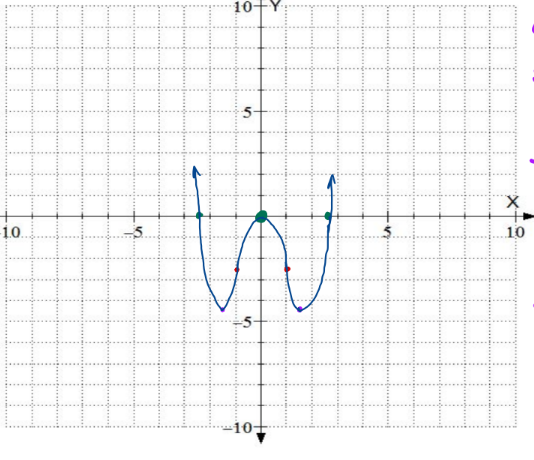
Execute the full 7-step curve sketching process for the even polynomial function:
Test for even symmetry: f(−x)=f(x). Find critical numbers by solving f′(x)=2x3−6x=0. Locate inflection points by solving f′′(x)=6x2−6=0. (See Summary of Curve Sketching.)
Answer:
Step-by-Step Execution
- Name the Governing Protocol: The Master 7-Step Curve Sketching Protocol: (Codified in Summary of Curve Sketching.)
- Step 1: Domain & Continuity:
As a polynomial, the domain is all real numbers:
Domain: (−∞,∞)
- Step 2: Intercepts:
- y-intercept: f(0)=21(0)4−3(0)2=0⟹(0,0).
- x-intercepts: Set f(x)=0:
x2(21x2−3)=0⟹x=0orx2=6⟹x=±6≈±2.45Intercepts: (0,0), (6,0), and (−6,0).
- Step 3: Symmetry:
f(−x)=21(−x)4−3(−x)2=21x4−3x2=f(x)The function is even; the graph is completely symmetric across the vertical y-axis.
- Step 4: Asymptotes & End Behavior: No vertical, horizontal, or slant asymptotes. As x→±∞, the leading term 21x4→∞. Both arms open upward toward +∞.
- Step 5: First Derivative (Monotonicity & Extrema):
f′(x)=2x3−6x=2x(x2−3)Setting f′(x)=0 yields critical numbers: x=−3≈−1.73, x=0, and x=3≈1.73.
- On (−∞,−3): f′(x)<0⟹ Decreasing (↘).
- On (−3,0): f′(x)>0⟹ Increasing (↗).
- On (0,3): f′(x)<0⟹ Decreasing (↘).
- On (3,∞): f′(x)>0⟹ Increasing (↗). Extrema coordinates:
- Relative Minimums: At x=±3, f(±3)=21(9)−3(3)=4.5−9=−4.5⟹(−3,−4.5) and (3,−4.5).
- Relative Maximum: At x=0, f(0)=0⟹(0,0).
- Step 6: Second Derivative (Concavity & Inflection Points):
f′′(x)=6x2−6=6(x2−1)=6(x−1)(x+1)Setting f′′(x)=0⟹x=−1 and x=1.
- On (−∞,−1)∪(1,∞): f′′(x)>0⟹ Concave Upward (∪).
- On (−1,1): f′′(x)<0⟹ Concave Downward (∩).
Inflection coordinates:
f(±1)=21(1)−3(1)=−2.5⟹(−1,−2.5)and(1,−2.5)
- Step 7: Information Consolidation Table & Final Sketch:
| Feature | Coordinate Point | Slope f′(x) | Concavity f′′(x) | Geometric Action |
|---|---|---|---|---|
| x-Intercept | (−2.45,0) | Negative | Positive (∪) | Descend through axis in cup shape |
| Relative Min | (−1.73,−4.5) | 0 (Horizontal) | Positive (∪) | Smooth valley trough |
| Inflection Point | (−1,−2.5) | Positive | 0 (Transition) | Switch curvature to cap shape |
| Relative Max | (0,0) | 0 (Horizontal) | Negative (∩) | Smooth peak summit at origin |
| Inflection Point | (1,−2.5) | Negative | 0 (Transition) | Switch curvature back to cup shape |
| Relative Min | (1.73,−4.5) | 0 (Horizontal) | Positive (∪) | Smooth symmetric valley trough |
| x-Intercept | (2.45,0) | Positive | Positive (∪) | Ascend through axis into +∞ |
Draw a smooth, symmetric "W"-shaped curve flowing through these coordinates:
Practice Problem 7
Execute the full 7-step curve sketching process for the transcendental function:
Evaluate the left-end limit limx→−∞(3−x)ex using L'Hôpital's Rule on e−x3−x. Use the Product Rule for both derivatives. (See Summary of Curve Sketching.)
Answer:
Step-by-Step Execution
- Name the Governing Protocol: The Master 7-Step Curve Sketching Protocol: (Codified in Summary of Curve Sketching.)
- Step 1: Domain & Continuity:
Both (3−x) and ex are defined everywhere:
Domain: (−∞,∞)
- Step 2: Intercepts:
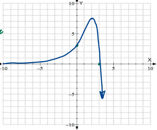
- y-intercept: g(0)=(3−0)e0=3(1)=3⟹(0,3).
- x-intercept: (3−x)ex=0. Since ex>0 for all real x, 3−x=0⟹x=3⟹(3,0).
- Step 3: Symmetry:
g(−x)=(3−(−x))e−x=(3+x)e−x=±g(x)No symmetry.
- Step 4: Asymptotes & End Behavior:
- No vertical asymptotes.
- Right End Behavior (x→∞):
x→∞lim(3−x)ex=(−∞)(∞)=−∞
- Left End Behavior (x→−∞):
x→−∞lim(3−x)ex=x→−∞lime−x3−x[∞∞]Apply L'Hôpital's Rule:x→−∞lim−e−x−1=x→−∞lime−x1=x→−∞limex=0This establishes a Horizontal Asymptote at y=0 along the negative x-axis.
- Step 5: First Derivative (Monotonicity & Extrema):
Apply the Product Rule:
g′(x)=(−1)ex+(3−x)ex=(2−x)exSetting g′(x)=0⟹2−x=0⟹x=2.
- On (−∞,2): g′(x)>0⟹ Increasing (↗).
- On (2,∞): g′(x)<0⟹ Decreasing (↘).
- Relative Maximum: Changes from increasing to decreasing at x=2:
g(2)=(3−2)e2=e2≈7.39⟹(2,e2)
- Step 6: Second Derivative (Concavity & Inflection Points):
Differentiate g′(x)=(2−x)ex:
g′′(x)=(−1)ex+(2−x)ex=(1−x)exSetting g′′(x)=0⟹1−x=0⟹x=1.
- On (−∞,1): g′′(x)>0⟹ Concave Upward (∪).
- On (1,∞): g′′(x)<0⟹ Concave Downward (∩).
- Point of Inflection: Concavity flips at x=1:
g(1)=(3−1)e1=2e≈5.44⟹(1,2e)
- Step 7: Information Consolidation Table & Final Sketch:
| Feature | Coordinate Point | Slope g′(x) | Concavity g′′(x) | Geometric Action |
|---|---|---|---|---|
| Horizontal Asymptote | y=0 as x→−∞ | 0+ | Positive (∪) | Emerges asymptotically along the negative x-axis |
| Inflection Point | (1,5.44) | Positive | 0 (Transition) | Switch from cup shape to bowl cap |
| y-Intercept | (0,3) | Positive (2) | Positive (1) | Cross vertical axis climbing steeply |
| Relative Maximum | (2,7.39) | 0 (Horizontal) | Negative (∩) | Smooth crest peak summit |
| x-Intercept | (3,0) | Negative (−e3) | Negative (∩) | Plunge through horizontal axis into −∞ |
Explore the interactive model in Desmos:
Annotated solution curve:
Practice Problem 8
Execute the full 7-step curve sketching process for the symmetric rational function:
Factor the denominator: x2−4=(x−2)(x+2) to identify the vertical asymptotes. Compare degrees of numerator and denominator for the horizontal asymptote. (See Summary of Curve Sketching.)
Answer:
Step-by-Step Execution
- Name the Governing Protocol: The Master 7-Step Curve Sketching Protocol: (Codified in Summary of Curve Sketching.)
- Step 1: Domain & Discontinuities:
Set denominator to zero:
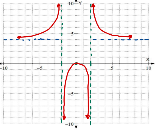
x2−4=0⟹x=±2Domain: (−∞,−2)∪(−2,2)∪(2,∞)
- Step 2: Intercepts:
- y-intercept: h(0)=0−44(0)2=0⟹(0,0).
- x-intercept: 4x2=0⟹x=0⟹(0,0).
- Step 3: Symmetry:
h(−x)=(−x)2−44(−x)2=x2−44x2=h(x)The function is even; symmetric with respect to the y-axis.
- Step 4: Asymptotes & End Behavior:
- Vertical Asymptotes: At x=−2 and x=2, the numerator is 4(4)=16=0:
Vertical Asymptotes at x=−2andx=2
- As x→2+, h(x)→+∞; as x→2−, h(x)→−∞.
- As x→−2+, h(x)→−∞; as x→−2−, h(x)→+∞.
- Horizontal Asymptote: Equal degrees (n=m=2):
x→±∞limx2−44x2=x→±∞lim1−x244=4⟹y=4
- Vertical Asymptotes: At x=−2 and x=2, the numerator is 4(4)=16=0:
- Step 5: First Derivative (Monotonicity & Extrema):
Quotient Rule:
h′(x)=(x2−4)2(8x)(x2−4)−(4x2)(2x)=(x2−4)28x3−32x−8x3=(x2−4)2−32xSetting h′(x)=0⟹−32x=0⟹x=0. Denominator is always positive when defined (x=±2):
- On (−∞,−2)∪(−2,0): h′(x)>0⟹ Increasing (↗).
- On (0,2)∪(2,∞): h′(x)<0⟹ Decreasing (↘).
- Relative Maximum: Changes +→− at x=0⟹(0,0).
- Step 6: Second Derivative (Concavity & Inflection Points):
Differentiate h′(x)=(x2−4)2−32x:
h′′(x)=(x2−4)4(−32)(x2−4)2−(−32x)⋅2(x2−4)(2x)=(x2−4)4(x2−4)[−32(x2−4)+128x2]=(x2−4)396x2+128The numerator 96x2+128>0 is strictly positive for all real x. Thus, h′′(x)=0 anywhere. Sign is dictated entirely by (x2−4):
- On (−∞,−2)∪(2,∞): x2−4>0⟹h′′(x)>0⟹ Concave Upward (∪).
- On (−2,2): x2−4<0⟹h′′(x)<0⟹ Concave Downward (∩).
- Inflection Points: None. Although concavity flips across x=±2, these values are vertical asymptotes that do not belong to the domain.
- Step 7: Information Consolidation Table & Final Sketch:
| Region / Coordinate | Feature Type | Monotonicity | Concavity | Visual Sketching Action |
|---|---|---|---|---|
| (−∞,−2) | Left Wing | Increasing (↗) | Concave Up (∪) | Slide along y=4 from left; curve upward to +∞ at x=−2 |
| x=−2 | Vertical Asymptote | Boundary | Undefined | Draw dashed line x=−2 |
| (−2,0) | Central Left | Increasing (↗) | Concave Down (∩) | Emerge from −∞; climb upward toward peak |
| (0,0) | Relative Maximum | Peak (h′=0) | Concave Down (∩) | Crest smoothly at origin |
| (0,2) | Central Right | Decreasing (↘) | Concave Down (∩) | Descend downward toward −∞ |
| x=2 | Vertical Asymptote | Boundary | Undefined | Draw dashed line x=2 |
| (2,∞) | Right Wing | Decreasing (↘) | Concave Up (∪) | Plunge from +∞ at x=2; flatten rightward toward y=4 |
Explore the interactive model in Desmos:
Annotated solution curve:
📅 Regroup 3
- Peer Audit of Final Sketches: Exchange curve sketches with a peer. Check three items:
- Did they draw asymptotes as dashed lines with arrows?
- Does the curve respect the concavity changes, or does it look like a series of straight line segments?
- Are local extrema clearly positioned as peaks/valleys with horizontal tangent slopes (f′=0)?
📅 Synthesis Wrap-up
- Core Takeaways:
- Curve sketching is not about memorizing shapes; it is the systematic translation of algebraic and differential properties into coordinate space.
- The first derivative tells you direction (↗,↘); the second derivative tells you curvature (∪,∩).
- Never declare an inflection point without verifying both continuity at c and a genuine sign change in f′′(x)!
- Homework & Preview:
- Complete Knewton Alta: The First Derivative Test and Concavity and Curve Sketching.
- Next Session preview: In Session 17 - Numerical Methods, we will study what happens when algebraic factoring fails completely, using tangent lines to construct Newton's Method for finding roots iteratively.