Absolute and Relative Extrema

Core Definition

Let $f$ be a function with domain $D$ .

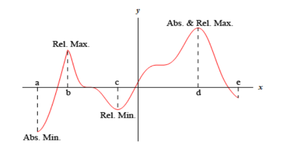
Absolute (Global) Maximum: $f$ has an absolute maximum at $c$ if $f(c) \ge f(x)$ for all $x \in D$ . The real number $f(c)$ is the absolute maximum value.
Absolute (Global) Minimum: $f$ has an absolute minimum at $c$ if $f(c) \le f(x)$ for all $x \in D$ . The real number $f(c)$ is the absolute minimum value.
Relative (Local) Maximum: $f$ has a relative maximum at $c$ if there exists an open interval $I$ containing $c$ such that $f(c) \ge f(x)$ for all $x \in I \cap D$ .
Relative (Local) Minimum: $f$ has a relative minimum at $c$ if there exists an open interval $I$ containing $c$ such that $f(c) \le f(x)$ for all $x \in I \cap D$ .

Concept Explanation

When reporting optimization results in engineering and calculus, precision in language is essential:

Location ( $x$ -coordinate): Specifies where the extremum occurs (e.g., "the maximum occurs at location $x = 4\text{ meters}$ ").
Extreme Value ( $y$ -coordinate): Specifies the actual quantity or height attained by the function (e.g., "the maximum bending moment value is $66\text{ kN}\cdot\text{m}$ ").
Extreme Point ( $xy$ -coordinate pair): Combines location and value as an ordered pair $(c, f(c))$ on the Cartesian coordinate plane.

Example: If f(3) = 15 is the peak of the curve:
- The maximum location is x = 3
- The maximum value is 15
- The maximum point is (3, 15)

The Endpoint Rule

Relative (local) extrema can NEVER occur at endpoints of a domain interval.

By definition, a relative extremum requires an open neighborhood $(c - \delta, c + \delta)$ centered at $c$ that lies entirely within the domain of the function, allowing values to be compared on both the left and the right of $c$ .
At a boundary endpoint (such as $x = a$ or $x = b$ in $[a, b]$ ), points exist only on one side. Therefore, interval boundaries can qualify as absolute extrema, but they are mathematically disqualified from being relative extrema.

Uniqueness of Values: A function can have at most one absolute maximum value and at most one absolute minimum value over its domain.
Multiplicity of Locations: An absolute extreme value can occur at multiple locations. For example, the function $f(x) = \sin(x)$ on $[0, 2\pi]$ attains its absolute maximum value of $1$ at location $x = \frac{\pi}{2}$ , and its absolute minimum value of $-1$ at location $x = \frac{3\pi}{2}$ . Over the entire real line $(-\infty, \infty)$ , $\sin(x)$ achieves its absolute maximum value of $1$ at infinitely many locations $x = \frac{\pi}{2} + 2\pi k$ ( $k \in \mathbb{Z}$ ).
Non-Existence: Absolute extrema do not necessarily exist. A function can fail to attain an absolute maximum or minimum if the domain is open (approaching a hole/open boundary) or if the function grows without bound ( $\lim_{x \to \pm\infty} f(x) = \pm\infty$ or vertical asymptotes).

Aerospace Wing Pitch Aerodynamics: Aircraft wings are profiled to produce a lift coefficient $C_L(\alpha)$ as a function of angle of attack $\alpha$ . The absolute maximum of $C_L(\alpha)$ defines the critical stall point ( $C_{L,\max}$ ). Flight control computers lock the trim elevator limits strictly below this angle to ensure aerodynamic controllability and prevent boundary layer separation stall.
Power Electronics Maximum Power Point Tracking (MPPT): Solar photovoltaic panels exhibit non-linear power-voltage curves $P(V) = V \cdot I(V)$ . Modern microinverters execute iterative hill-climbing algorithms to drive the terminal voltage directly to the location of the absolute maximum power output, optimizing energy harvesting under shifting cloud cover.
Structural Engineering Load Envelopes: In bridge structural design, civil engineers compute the envelope of internal shear stresses $V(x)$ under rolling wheel loads. Locating both the absolute maximum (highest compressive shear) and absolute minimum (highest tensile shear) determines the cross-sectional steel web thickness required along the span.

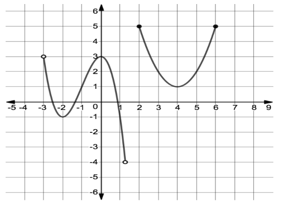
Consider the piecewise curve defined on $[-3, 6]$ shown below:

Determine all relative and absolute extrema (values and locations):

Solution

Relative Maxima:
- $y = 3$ at location $x = 0$ . (This is a smooth interior peak where the function is larger than all neighboring points on both sides).
- Endpoint check: The points $x = 2$ and $x = 6$ reach $y = 5$ , but $x = 6$ is an endpoint (no two-sided neighborhood), and $x = 2$ has domain points only for $x \ge 2$ (the branch to the left terminates with an open circle at $(1.25, -4)$ and is discontinuous). Therefore, there is only one relative maximum.
Absolute Maximum:
- Value: $5$ , attained at two locations: $x = 2$ and $x = 6$ . Both points have solid dots, meaning $f(2) = 5$ and $f(6) = 5$ are explicitly reached.
Relative Minima:
- Value: $-1$ at location $x = -2$ .
- Value: $1$ at location $x = 4$ . Both points are smooth interior valleys with valid two-sided open neighborhoods.
Absolute Minimum:
- Does not exist (DNE).
- Analysis: The curve drops downward toward $y = -4$ as $x \to 1.25^-$ on the left branch, terminating in an open circle at $(1.25, -4)$ . Because this lowest point is excluded, the function values get arbitrarily close to $-4$ but never actually attain $-4$ . Since no lower point exists and $-4$ is not in the range, the function has no absolute minimum.

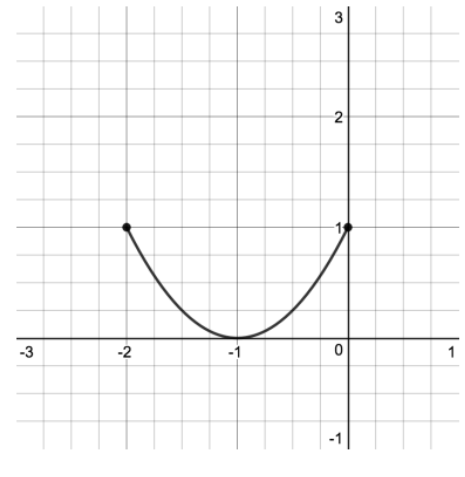
Identify the absolute and relative extrema for $f(x) = (x + 1)^2$ on the closed interval $[-2, 0]$ :

Solution

Differentiate: $f'(x) = 2(x + 1) = 0 \implies x = -1$ .
Candidate Values:
- Left Endpoint: $f(-2) = (-2 + 1)^2 = 1$ .
- Interior Critical Point: $f(-1) = (-1 + 1)^2 = 0$ .
- Right Endpoint: $f(0) = (0 + 1)^2 = 1$ .
Classification:
- Absolute Minimum: Value $0$ at location $x = -1$ .
- Relative Minimum: Value $0$ at location $x = -1$ (interior valley with a full two-sided neighborhood).
- Absolute Maximum: Value $1$ at locations $x = -2$ and $x = 0$ .
- Relative Maxima: None. (The highest peaks occur strictly at the boundaries $x = -2$ and $x = 0$ , which are endpoints and are disqualified by the Endpoint Rule).