Closed Interval Method

Core Definition

The Closed Interval Method is an exact analytical algorithm used to locate the absolute maximum and absolute minimum values of a continuous function $f(x)$ on a closed interval $[a, b]$ . Because absolute extrema can occur only at interior critical numbers or at boundary endpoints, the method evaluates the original function $f(x)$ across all candidate points and directly compares their heights ( $y$ -values).

Concept Explanation

1. The 5-Step Closed Interval Method Pipeline

When a function satisfies the preconditions of the Extreme Value Theorem, execute the following 5-step pipeline:

Step 1: Check Preconditions (Continuity on [a, b])
                  |
Step 2: Differentiate (Compute f'(x))
                  |
Step 3: Find & Filter Interior Critical Numbers (c in (a, b) where f'(c)=0 or DNE)
                  |
Step 4: Evaluate Original Function f(x) at:
        - Surviving interior critical numbers: f(c_1), f(c_2), ...
        - Left boundary endpoint: f(a)
        - Right boundary endpoint: f(b)
                  |
Step 5: Compare Heights:
        - Highest value  --> Absolute Maximum Value
        - Lowest value   --> Absolute Minimum Value

2. Common Pitfalls to Avoid

Pitfall 1: The Derivative Evaluation Trap: Never substitute candidate points back into the derivative $f'(x)$ . Substituting critical numbers into $f'(x)$ yields $0$ or undefined. Always evaluate the original function $f(x)$ to find the physical heights ( $y$ -values).
Pitfall 2: Forgetting Endpoints: Absolute extrema frequently occur at the boundaries $x = a$ or $x = b$ , where $f'(x) \neq 0$ . Neglecting endpoint evaluations can cause you to miss the true global maximum or minimum.
Pitfall 3: Failing to Filter Candidates: Only critical numbers located strictly inside the open interval $(a, b)$ are valid candidates. Any solutions to $f'(x) = 0$ outside $(a, b)$ must be discarded.
Pitfall 4: Overlooking Singular Points ( $f'(x) \text{ DNE}$ ): Always check whether the denominator of $f'(x)$ can equal zero within $(a, b)$ (e.g., fractional exponents such as $x^{2/3}$ or $x^{1/3}$ ).

Engineering Applications

Civil Structural Beam Bending Moments: Reinforced concrete bridge beams spanning $x \in [0, L]$ experience internal bending moment distributions $M(x)$ . Civil engineers use the Closed Interval Method to compare moments at support piers ( $x = 0, L$ ) against internal critical moment sections ( $M'(x) = 0$ ), ensuring rebar steel reinforcement is placed at the absolute peak bending stress location.
Transistor Thermal Duty-Cycle Analysis: Power semiconductor devices (such as GaN MOSFETs) experience thermal junction heating $T(t)$ over a periodic switching cycle $[0, t_{\text{cycle}}]$ . Electronic systems engineers apply the Closed Interval Method to verify that the absolute peak junction temperature does not breach the silicon thermal damage ceiling.
Subsea Pipeline Pressure Cycling: Marine petroleum pipelines spanning a seabed elevation profile $z(s)$ over total pipeline length $s \in [0, L_{\text{pipe}}]$ must withstand hydrostatic burst pressure. Engineers evaluate pipeline wall stresses at intermediate high/low points and boundary manifolds using closed-interval optimization.

Example Problems

Example 1: Polynomial on a Closed Interval

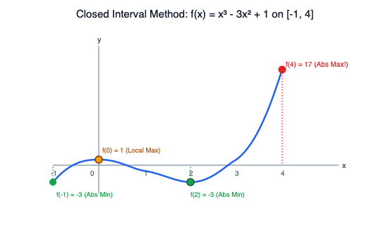
Find the absolute maximum and minimum values of $f(x) = x^3 - 3x^2 + 1$ on the closed interval $[-1, 4]$ :

Solution

Check Continuity: $f(x)$ is a polynomial, so it is continuous on $[-1, 4]$ . The EVT applies.
Differentiate: $f'(x) = 3x^2 - 6x = 3x(x - 2)$
Locate and Filter Critical Numbers: Set $f'(x) = 0$ : $3x(x - 2) = 0 \implies x = 0 \quad \text{and} \quad x = 2$ Filter: Both $x = 0$ and $x = 2$ lie strictly inside the interior interval $(-1, 4)$ . Both are retained.
Evaluate Original Function $f(x)$ at All Candidates:
- Left Endpoint ( $x = -1$ ): $f(-1) = (-1)^3 - 3(-1)^2 + 1 = -1 - 3 + 1 = -3$
- First Critical Number ( $x = 0$ ): $f(0) = (0)^3 - 3(0)^2 + 1 = 1$
- Second Critical Number ( $x = 2$ ): $f(2) = (2)^3 - 3(2)^2 + 1 = 8 - 12 + 1 = -3$
- Right Endpoint ( $x = 4$ ): $f(4) = (4)^3 - 3(4)^2 + 1 = 64 - 48 + 1 = 17$
Compare and Conclude:
- Absolute Maximum Value: $17$ at location $x = 4$ .
- Absolute Minimum Value: $-3$ at locations $x = -1$ and $x = 2$ .

Example 2: Function with a Cusp on a Closed Interval

Find the absolute extrema of $g(x) = 2x - 3x^{2/3}$ on $[-1, 8]$ :